Gentle introduction to graph neural networks and graph convolutional networks

Decoding the complexity of graph data with neural networks.

Graph neural networks (GNNs) have emerged as a powerful tool for processing data structured as graphs, offering a significant leap in machine learning. These networks are designed to handle complex, non-Euclidean structured data, such as social networks, molecular structures, and supply chains, often represented as graphs. GNNs pass messages or information between nodes in a graph, enabling the understanding and interpreting of complex relationships and dependencies within the data.

In the realm of GNNs, one of the core approaches is using Graph Convolutional Networks (GCNs). Drawing parallels with the operation of traditional convolutional neural networks (CNNs) used in image and text processing, GCNs apply a similar principle to graph data. They aggregate information from a node’s neighborhood and transform it through multiple layers deep neural network, creating a new representation of the node that captures its features and the context of its surroundings. This unique approach allows GCNs to handle the complexity and diversity inherent in graph data, opening up new data analysis and prediction possibilities.

What are neural networks?

Neural networks, often referred to as artificial neural networks (ANNs) are computing systems inspired by the human brain’s biological neural networks. They are the backbone of artificial intelligence (AI) and machine learning (ML), designed to simulate how humans learn and make decisions. Neural networks comprise interconnected layers of nodes, or “neurons,” which process information using dynamic state responses to external inputs.

The power of neural networks lies in their ability to understand complex patterns and relationships within data. They can handle large amounts of data, learn from it, and improve their performance over time. They are widely used in various applications, including image and speech recognition, natural language processing, and predictive analytics. Their ability to learn and adapt makes them crucial in AI and ML.

What is graph processing, and what are graph neural networks?

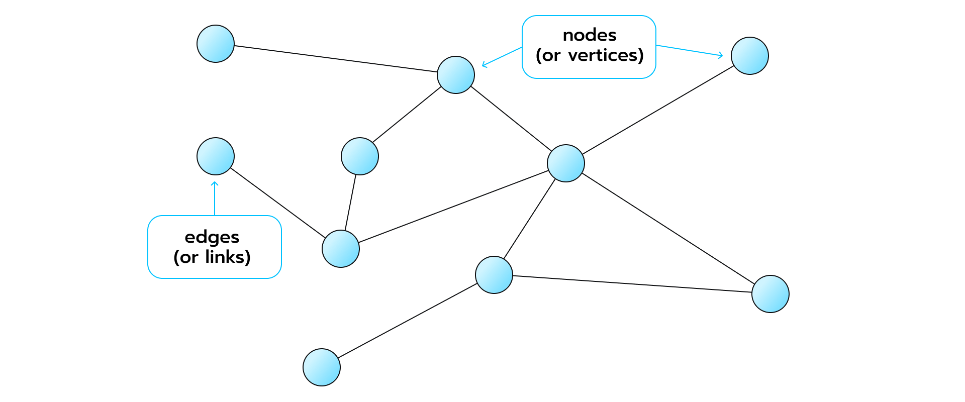
Graphs are data structures that consist of vertices (nodes) and edges (links). Mathematically they’re defined as G = (E, V), but you’re probably more familiar with them looking like this:The edges can be directed or not, depending on whether there are directional dependencies between the edge weights and the data points.

Graphs are essential because lots of things in the real world can be represented by them, such as organizational hierarchies, social networks, complex relationships, molecules (where atoms can be visualized as nodes and chemical bonds as edges), protein-protein-interaction systems, supply chains, knowledge graphs, etc. As a data structure, they possess tremendous expressive power.

These data structures are profoundly simpler than graphs that might have arbitrary size, multimodal features, complex topology, and no fixed node ordering.

Different complex graph structures and various deep learning and neural network and methods have been proposed to address this. In this article, we’ll cover one of the core deep learning approaches to processing complex graph structures in data: graph convolutional networks.

Let’s get to it.

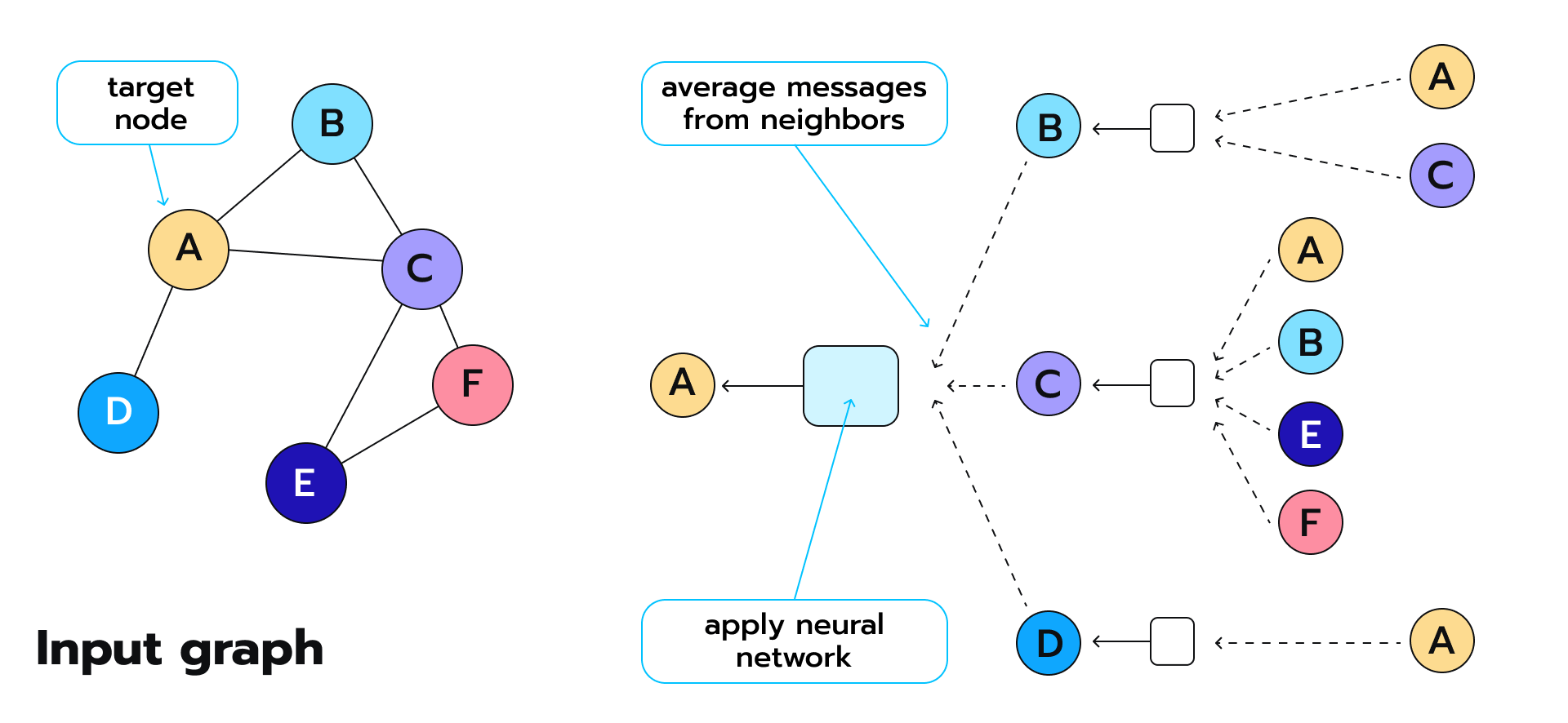
Before we dig into graph processing, we should talk about the message passing the whole graph itself. Or message passing? Generally, message passing layer that each node in a graph sends information about itself to its neighbors and receives messages from them to update its status and understand its environment.

For example, in a basic label propagation algorithm, every node in the output graph structure starts with some initial state, receives a signal from its neighbors to update it, and then runs the same process in the next iteration but, this time, with an updated starting value. The number of these iterations (timesteps) is a tunable hyperparameter.

Graph neural networks do the same thing, except not just for label values – they spread messages about the entire input data vectors. If label propagation can be compared to simple label smoothing, then what a Graph neural network does can be considered feature smoothing.

How does a graph convolutional network model work?

First, each node gets information about all its connected nodes’ features and applies an aggregation function such as sum or average to these values, which ensures that all representations come out of the same size. Whatever function we end up choosing, it must be permutation and order invariant. This is crucial.

Afterward, the resulting vector is passed through a dense neural network layer (which means it is multiplied by some matrix). Then a non-linear activation function is used on top of that activation function to get a new vector representation.

Next, we keep looping through these three steps:

• For every node, aggregate its neighbors’ vectors (now the updated ones).
• Pass the resulting value through a dense neural net layer.
• Apply non-linearity.

We do this as many times as our network has layers.

It’s important to remember that the nodes in Graph neural networks will have a different representation at each layer. Graph neural networks

• At the 0-th layer, they will be the same as the node’s features.
• At layer k, to compute a representation for a node, we’ll go over its neighbors, take their representations from the previous layer k -1, and average those together. Then we’ll transform them using a parameter matrix and add the node’s messages from k -1. The resulting value will be passed through a non-linear function such as ReLU.
• Finally, after the node’s representation has gone through all the transformations in the hidden layers, we’ll get the final embedding.

There are two tunable parameter matrices that we apply at each node feature matrix and layer – one to transform the values of the two neighboring nodes into neighboring node features, that are represented from k -1, and another to transform the aggregated messages from the adjacent nodes (again from k -1). graph neural networks

During training, we’re figuring out the optimal way to enrich the information a node learns about itself. It boils down to how much of a non-linear transformation we want to do over the node’s feature vectors vs. how much of a modification we need to apply to the neighbors’ feature vectors. Depending on the matrices we use, we can make the node focus entirely on the information about itself and ignore the messages from its environment, the other way around, or a little bit of both, whichever helps us get the best predictions.

Note: the more timesteps we set up, the farther the signal from our nodes will travel. And suppose we’re dealing with an average-sized graph, and the messages do 3 to 5 hops through the edges. In that case, that will be enough for a node to affect the representation of pretty much every other node in the same graph (to a varying extent, that depends on the distance).If all this sounds familiar, here’s why: In standard convnets, we typically slide a convolutional operator over a pixel grid and process one sub-patch of an image at a time. We combine and transform pixel value information to create new representations, and, in a way, we treat groups of pixels as neighborhoods of nodes. So, overall, the logic behind Graph spatial convolutional networks is highly similar to that of all conventional neural nets: the output of spatial convolutional neural networks used at one layer is fed to the next as input. However, there are some significant distinctions too.

1. In Graph convolutional networks, we run the preprocessing step of aggregating the values of a node’s neighbors and averaging them out on every layer.
2. The local network neighborhood of a node will define the data structure consisting of its computational Graph, which will be different from that of all other vertices. Therefore, every node will have its neural network architecture that will capture and reflect the structure global context of its environment.

We can also choose to train the networks unsupervised, using random walks, node proximity, graph factorization, etc., as a loss function.

In graph neural networks, how many layers we have puts an upper limit on how far the messages from each node can travel through the connections of the entire graph data and structure. In a two-layer network, for instance, we’ll run message passing twice, so the signal will only do two hops from the source node and won’t be affected by the info outside the subgraph. If long-range dependencies are crucial to the problem, we must use more layers.

Graph neural network limitations

The field is young, and despite the impressive breakthroughs Graph neural networks have achieved on some datasets (state-of-the-art performances on graph node image classification alone, link prediction, and graph node classification alone), there are still flaws in them that the community is struggling to fix. Here are the two major concerns:

Graph neural networks, in general, are not robust to noise. Even through simple feature perturbations and addition (or deletion) of edges, we can flip all the classifications a Graph neural network produces.

Graph structure and graph structured data

Graph convolutional networks sometimes fail to distinguish between simple graph structures and graph-structured data with a slightly different adjacency matrix if their input features are uniform. This presents a considerable challenge in downstream tasks such as social network analysis and graph analysis such as graph classification.

The structure of a graph is defined by how its nodes and edges are arranged. This structure can be simple or complex, depending on the number of nodes and edges and their interconnectedness. For instance, a social network graph might have millions of nodes (people) and edges (relationships) with complex patterns of connections. On the other hand, a family tree graph would have a more straightforward hierarchical structure.

Understanding and leveraging graph structures and graph-structured data is a significant challenge in data science and machine learning. Traditional machine learning methods often struggle with this data type because they are designed for grid-like data structures (like images) or sequential data (like text). This is where graph neural networks, specifically Graph Convolutional Networks (GCNs), come into play. They are designed to work directly with graph structures, using node connections to extract meaningful features and make predictions. However, as mentioned earlier, they can struggle when the input features of graph datasets are uniform, highlighting the need for diverse and informative node features in graph-structured data.

To sum up

Though they’re quite new, Graph neural networks already have many applications in industry. At Pinterest, for example, a Graph neural network is used as an engine for a recommendation system, and according to Jure Leskovec (Pinterest’s Chief Scientist), it produces by far the best embeddings. Uber has recently published a post describing how a Graph neural network-based approach helps them give accurate recommendations for their UberEats service.

Other exciting applications include using a heterogeneous Graph neural network, Decagon, to discover and predict polypharmacy side effects and using a Graph Convolutional Policy Network (GCPN) for molecular graph generation.

Want to learn more about graph representation learning? Want to know how Graph neural networks can help you solve high-impact business problems? Reach out to our expert right now and get a free consultation.